Diffuse signal processing (DiSP) was first described as a method of signal decorrelation by Malcolm Hawksford in 2002 [1]. It is based on the synthesis of temporally diffuse impulses (TDIs), which are then convolved with the driving signal of each discrete loudspeaker in an array. The TDIs randomise the phase of each driving signal, thereby lowering the inter-channel correlation of the array.
I won’t go into a large amount of detail into the TDI generation process here, as an in-depth explanation is given in Malcolm’s paper. In this post I will give a quick overview of what TDIs look like in the time and frequency domains, and some brief analysis on their effect on audio.
A TDI is an impulse followed by an exponentially decaying noise tail. The phase of each frequency of the TDI is randomised, and an all-pass magnitude response is achieved by minimum phase equalisation. This avoids most of the timbral colouration affects that occur with other audio signal decorrelation methods, although care has to be taken in TDI generation to ensure the filters are not audible. The most common artefact is temporal smearing and ringing, which is caused by selecting too-long a decay time for the noise tail.
TDI generation incorporates a frequency-dependant exponential decay, where the decay time for each frequency is roughly proportional to its period, to try and eliminate this. As part of my Ph. D. project, a subjective test was designed to find the audible limits of decay time by frequency [2]. TDIs generated using those parameters have been found to perform well without generating significant audible artefacts, although recent tests have shown that adding transient detection during the convolution process improves audio quality significantly without impacting performance.
In this post we will generate two independent TDIs, examine them in the time and frequency domains and then analyse their low-frequency decorrelation performance with an acoustic simulation. Low frequency decorrelation is potentially useful tool in the reduction of low frequency amplitude nulls across audience areas due to comb-filtering.
Fig 1. shows the two generated TDIs in the time domain. TDIs for low frequency decorrelation are necessarily long in order to get the low frequency resolution necessary. Therefore it is important to use an appropriate decay time selection to reduce any temporal smearing.
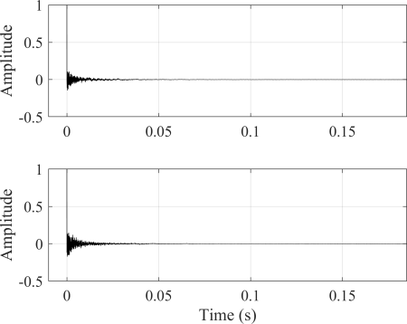
Fig. 1. Two independent TDIs in the time domain.
Fig. 2. shows the magnitude responses of the TDIs – they are flat due to the minimum phase equalisation technique described in Malcolm’s paper [1].
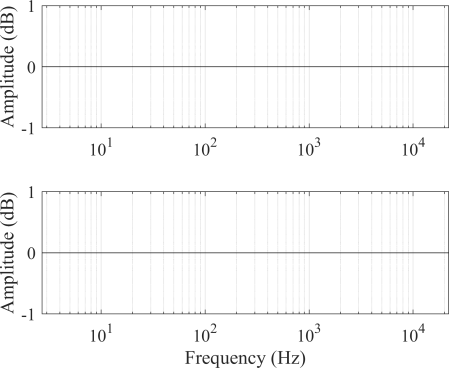
Fig. 2. Magnitude responses of the two TDIs shown in Fig 1.
Fig. 3. shows the wrapped phase responses of the TDIs. This illustrates that random phase variations in each TDI generated.
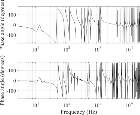
Fig. 3. Wrapped phase responses of the TDIs shown in Fig. 1. The length of the TDI dictates its frequency resolution. If TDIs are not long enough, there will not be enough variation in the phase at low frequencies due to inadequate resolution.
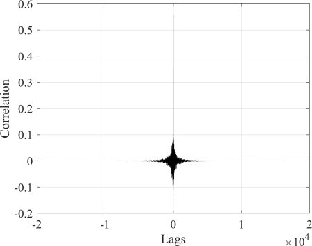
Fig. 4. shows the cross-correlation function of the two TDIs shown in Fig. 1. Peak correlation is when the two initial peaks are in alignment. Where they are not in alignment, i.e. when there is a time difference of arrival from each speaker, the correlation is low.
Next we will look at a very basic simulation with two sub-woofers positioned either side of a stage (black squares). A room of 10 x 10 meters was simulated. Fig. 5. shows the sound level distribution in dB around the audience area at 80 Hz. As we would expect, there are areas in the audience that suffer from amplitude nulls where destructive interference occurs. These nulls occur through out the frequency spectrum and their spatial distribution will change with frequency.
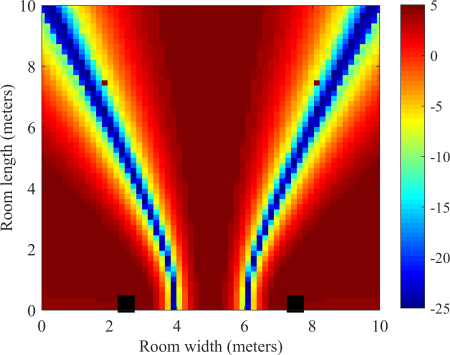 Fig. 5. A simple acoustic simulation of two sub-woofers postitioned either side of a stage without DiSP applied.
Fig. 6. shows the same simulation, but with the TDIs applied. The nulls areas seen in Fig. 5. still exist to a degree as the decorrelation is only partial. Crucially, the variance in sound level across the audience area is reduced by 43%.
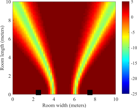
Fig. 6. A simple acoustic simulation of two sub-woofers positioned either side of a stage with DiSP applied.
This is very much a quick and dirty example. A large amount of my Ph. D. work has been focused on the optimisation of TDI generation to obtain the best results with minimal perceptual degradation to the audio. If you would like to see the level of audio degradation, I am happy to provide the TDIs used in this test – they should be downloadable as .wavs from the following link: TDIs.
To use, simply convolve with your audio file! A good exercise is to take a mono source and convolve it with the two TDIs to generate two independent channels, and then listen over headphones. The track will be externalised and appear to come from outside the headphones as opposed to internalised when the source is purely mono.
References:
[1] M.O.J. Hawksford, N. Harris, “Diffuse signal processing and acoustic source characterization for applications in synthetic loudspeaker arrays,” 112th Convention of the Audio Engineering Society, (2002, Apr), convention paper 5612
[2] Moore, J.B.; A.J. Hill. Dynamic diffuse signal processing for low frequency spatial variance minimization across wide audience areas. 143rd Convention of the Audio Engineering Society, New York, USA. October, 2017.
